

Conditional Formatting Tricks You Must Know)
Conditional Formatting Tricks You Must Know)
Learn the best Conditional Formatting tricks in Excel with practical examples. Highlight duplicates, overdue dates, top values, data bars, color scales, custom formulas, and more.
Focus Keyword: Conditional Formatting Tricks in Excel
Conditional Formatting Tricks You Must Know
When working with large datasets in Microsoft Excel, finding important information quickly can be challenging. That’s where Conditional Formatting becomes one of Excel’s most powerful features.
Instead of manually searching through hundreds or thousands of rows, Conditional Formatting automatically highlights important data based on rules you define.
Whether you’re tracking sales, managing inventory, analyzing employee performance, or building dashboards, mastering Conditional Formatting can make your spreadsheets more professional, interactive, and easier to understand.
In this guide, you’ll learn the best Conditional Formatting tricks every Excel user should know.
What is Conditional Formatting?
Conditional Formatting is an Excel feature that automatically changes the appearance of cells based on specified conditions.
For example, you can:
– Highlight high sales
– Mark overdue tasks
– Find duplicate records
– Display color scales
– Add data bars
– Show icons based on performance
This helps users identify trends and exceptions instantly.
Why Use Conditional Formatting?
Benefits include:
– Makes reports easier to read
– Highlights important values
– Detects errors quickly
– Improves dashboards
– Saves time
– Enhances decision-making
– Reduces manual checking
How to Apply Conditional Formatting
- Select your data range.
- Go to the Home tab.
- Click Conditional Formatting.
- Choose a rule type.
- Select formatting options.
- Click OK.
Your formatting updates automatically when the data changes.
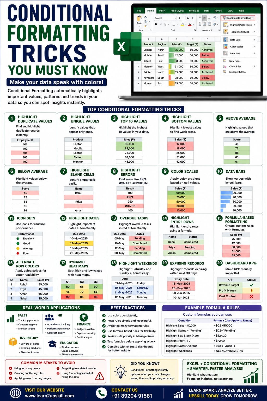
Trick 1: Highlight Duplicate Values
Duplicate records can affect reports and analysis.
Example
Employee ID
101
102
101
Use:
Home → Conditional Formatting → Highlight Cells Rules → Duplicate Values
Duplicates will be highlighted automatically.
Trick 2: Highlight Unique Values
You can also identify values that appear only once.
This is useful for:
– Customer IDs
– Invoice numbers
– Product codes
Trick 3: Highlight Top 10 Values
Quickly identify:
– Top-performing employees
– Highest sales
– Best products
Go to:
Top/Bottom Rules → Top 10 Items
You can change the number from 10 to any value.
Trick 4: Highlight Bottom Values
Find:
– Lowest sales
– Weak-performing products
– Low inventory
Use:
Top/Bottom Rules → Bottom 10 Items
Trick 5: Highlight Above Average
Excel can automatically highlight values above the average.
Useful for:
– High-performing salespeople
– Better-performing branches
– Outstanding student scores
Trick 6: Highlight Below Average
Similarly, identify values below average to spot areas that need improvement.
Trick 7: Highlight Blank Cells
Blank cells often indicate missing data.
Create a rule to highlight blanks so they can be filled before analysis.
Trick 8: Highlight Errors
Errors such as:
– #N/A
– #VALUE!
– #DIV/0!
can make reports unreliable.
Conditional Formatting helps identify these instantly.
Trick 9: Color Scales
Color scales assign different colors based on cell values.
Example:
– Green = High
– Yellow = Medium
– Red = Low
Perfect for sales reports and performance dashboards.
Trick 10: Data Bars
Data Bars display a horizontal bar inside each cell based on its value.
Benefits:
– Easy comparison
– Better visualization
– Quick performance review
Trick 11: Icon Sets
Excel includes built-in icons such as:
– Green arrows
– Yellow circles
– Red arrows
– Traffic lights
– Stars
– Flags
Ideal for KPI dashboards and performance tracking.
Trick 12: Highlight Dates
Automatically highlight:
– Today’s tasks
– Tomorrow’s deadlines
– Next week’s meetings
– Previous month’s records
Useful for project management and scheduling.
Trick 13: Highlight Overdue Tasks
Example
Task| Due Date| Status
Report| 12-Jan| Pending
If today’s date is later than the due date, Conditional Formatting can highlight the row in red.
Great for project tracking and task management.
Trick 14: Highlight Entire Rows
Instead of formatting a single cell, you can highlight the entire row using a custom formula.
Example:
Highlight all rows where:
Status = “Completed”
This makes reports much easier to scan.
Trick 15: Use Formula-Based Formatting
One of the most powerful features is creating your own rules.
Example Formula
=$C2=”Pending”
This can highlight all rows where the Status column contains “Pending”.
Other examples:
– Sales greater than ₹50,000
– Attendance below 75%
– Inventory less than 20
– Profit less than zero
Trick 16: Alternate Row Colors
Use Conditional Formatting to create zebra stripes for improved readability in large tables.
Trick 17: Dynamic Heat Maps
Combine Color Scales with your data to create heat maps that quickly reveal high and low values across a range.
Useful for:
– Sales analysis
– Exam scores
– Financial reports
– Performance metrics
Trick 18: Highlight Weekend Dates
Using a formula, you can highlight Saturdays and Sundays in project plans or attendance sheets.
This improves scheduling and planning.
Trick 19: Highlight Expiring Records
Monitor:
– License expiry
– Insurance renewal
– Employee contracts
– Membership validity
Highlight records expiring within the next 30 days.
Trick 20: Dashboard KPIs
Conditional Formatting can make dashboards more interactive.
Examples:
– Green = Target Achieved
– Yellow = Needs Attention
– Red = Below Target
This provides instant visual feedback.
Real-World Applications
Sales
– Highlight top-performing products
– Identify low-performing regions
– Show sales targets
HR
– Attendance tracking
– Performance reviews
– Contract expiry alerts
Finance
– Budget monitoring
– Expense tracking
– Profit analysis
Education
– Student performance
– Attendance reports
– Grade analysis
Inventory
– Low stock alerts
– Expiring products
– Overstock identification
Best Practices
– Use colors consistently.
– Avoid applying too many rules to the same range.
– Keep formatting simple and meaningful.
– Test custom formulas before applying them widely.
– Review rule priority using the Conditional Formatting Rules Manager.
Final Thoughts
Conditional Formatting is one of the most effective ways to make Excel reports easier to understand and more visually appealing. From highlighting duplicates and overdue tasks to building KPI dashboards and heat maps, it helps you spot important information instantly.
By mastering these tricks, you’ll create cleaner reports, improve decision-making, and work more efficiently—whether you’re a student, analyst, manager, or business professional.
At Learn2Upskill, we help students and professionals master Excel through practical tutorials, real-world projects, and career-focused training.
Visit: www.learn2upskill.com
Contact Us: +91 89204 91581
Turn Data into Insights with Smart Excel Skills.
You May Also Like
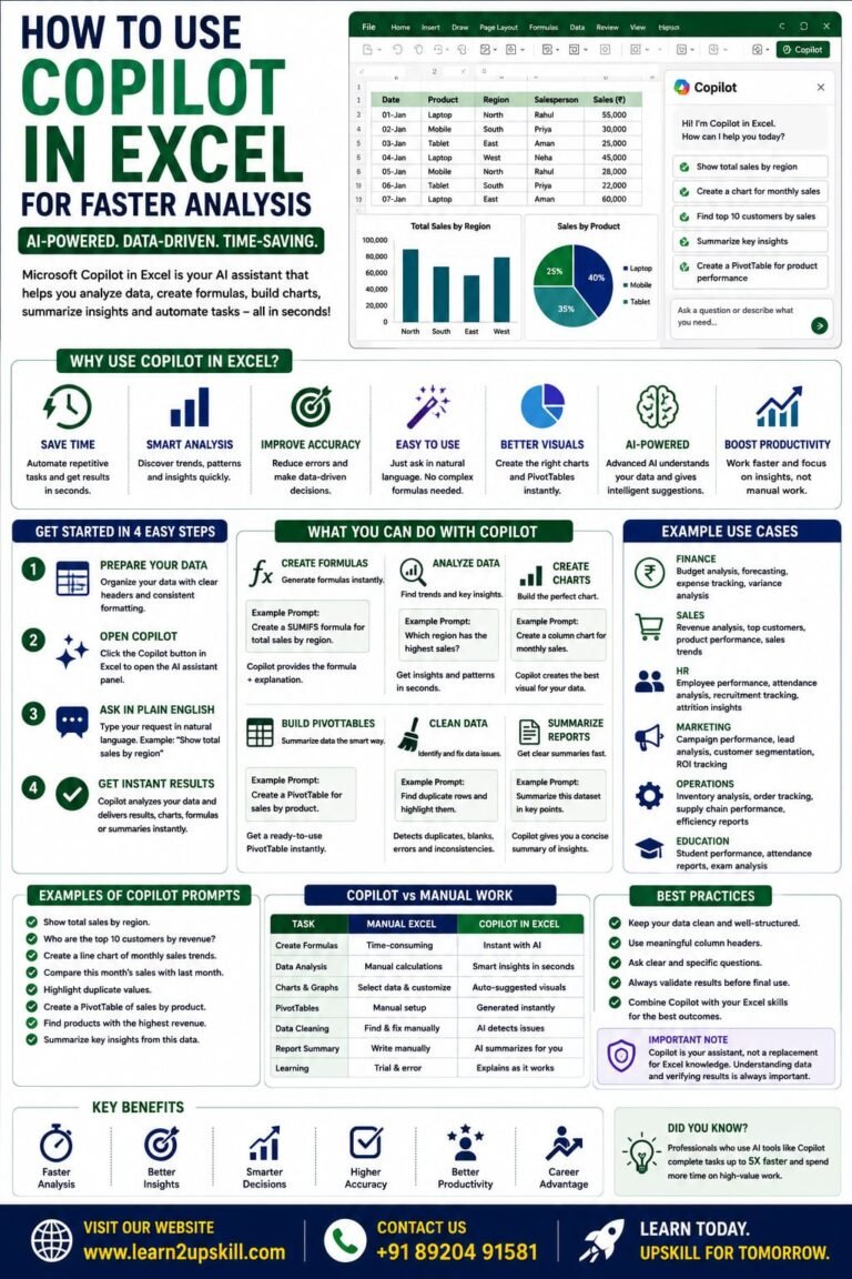
How to Use Copilot in Excel for Faster Analysis Learn how to use Microsoft Copilot in Excel to analyze data...
-
-
July 21, 2026
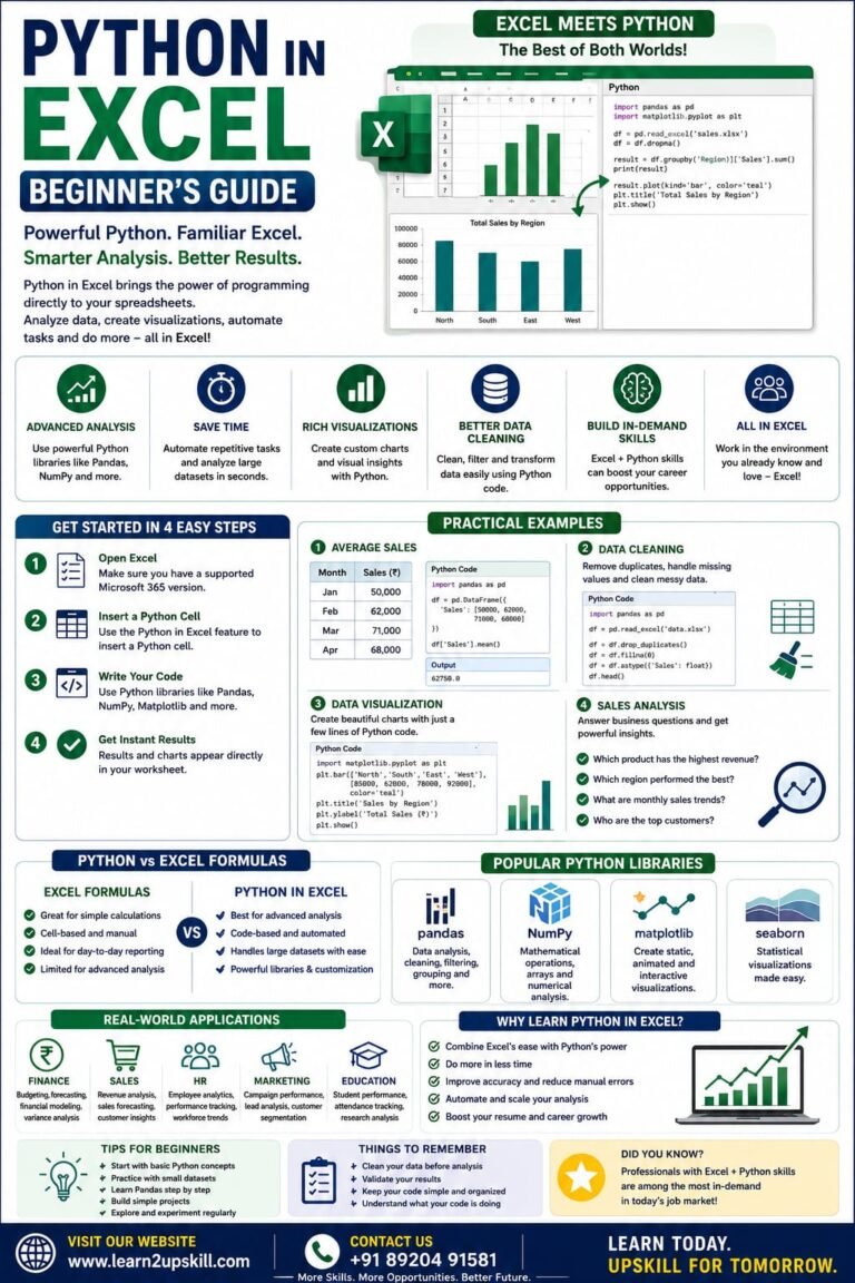
Python in Excel Learn how to use Python in Microsoft Excel with this beginner-friendly guide. Discover setup, syntax, examples, benefits,...
-
-
July 20, 2026
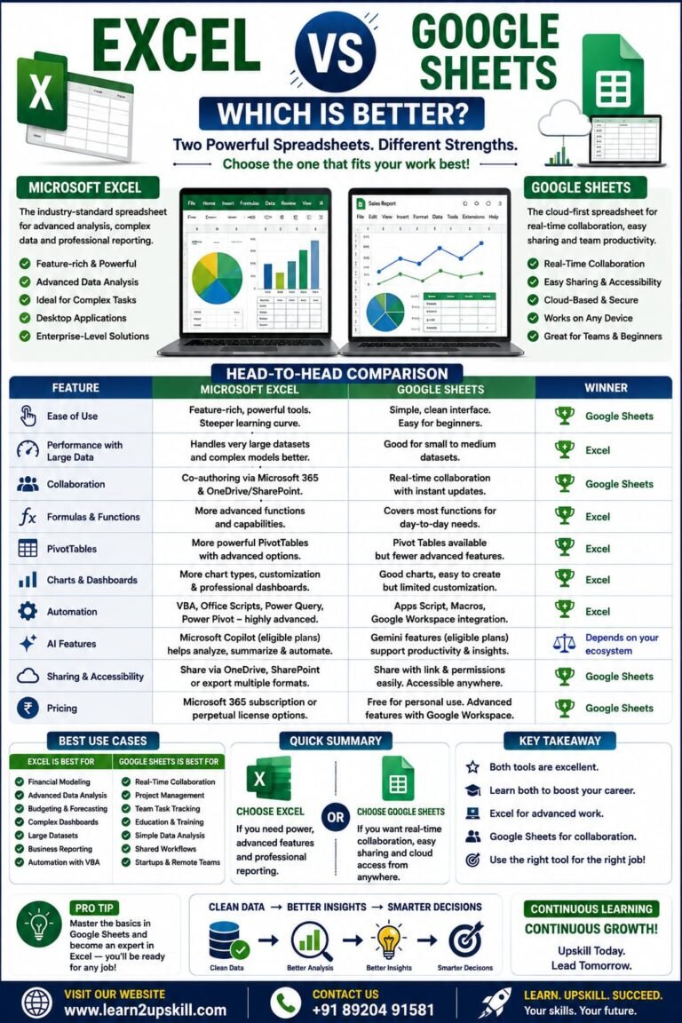
Excel vs Google Sheets: Which Is Better? Compare Microsoft Excel and Google Sheets in terms of features, performance, collaboration, AI...
-
-
June 10, 2026